Contact Force Law
Modia3D supports Collision Handling of objects that are defined with a contact material and (a) have a convex geometry, or (b) can be approximated by a set of convex geometries, or (c) have a concave geometry that is (automatically) approximated by its convex hull. When contact occurs, the response is computed with elastic (nonlinear) force/torque laws based on the penetration depth and the relative motion of the objects in contact. It is planned to optionally also support impulsive response calculation in the future.
This section is based on [4] with some improvements as used in the current version of Modia3D.
The current approach has several limitations that a user must know, in order that a simulation is successful:
- The current collision handling is designed for variable step-size integrators for systems that have realistic physical material behavior.
- Usually, a relative tolerance of $10^{-8}$ or smaller has to be used since otherwise a variable step-size integrator will typically fail. The reason is that the penetration depth is computed from the difference of tolerance-controlled variables and the precision will be not sufficient if a higher tolerance will be used because the penetration depth of hard contact materials is in the order of $10^{-5} .. 10^{-6}~ m$. A relative tolerancie of $10^{-5}$ might be used, if the heuristic elastic contact reduction factor is set to $k_{red} = 10^{-4}$ (see Material constants below).
- A reasonable reliable simulation requires that objects have only point contact, since otherwise the contact point can easily $jump$ between model evaluations and a variable step-size integrator will not be able to cope with this, so will terminate with an error. For this reason, all geometrical objects are slightly modified in various ways for the collision handling. Most important, all geometries are smoothed with a small sphere (e.g. with radius = 1mm) that is moved over all surfaces. Basically, this also means that if two objects are in contact, one of them should be a Sphere or an Ellipsoid.
Material constants
The response calculation uses the following material constants from the Solid material palette and from the Contact pair material palette.
YoungsModulusorEin [N/m^2]: Young's modulus of contact material ($\gt 0$).PoissonsRatioornu: Poisson's ratio of contact material ($0 \lt nu \lt 1$).coefficientOfRestitutionorcor: Coefficient of restitution between two objects ($0 \le cor \le 1$).slidingFrictionCoefficientormu_k: Kinetic/sliding friction force coefficient between two objects ($\ge 0$).rotationalResistanceCoefficientormu_r: Rotational rolling resistance torque coefficient between two objects ($\ge 0$).
Additionally, the response calculation is changed at small relative velocities and relative angular velocities. This region is defined by the following constants:
vsmallin [m/s]: Used for regularization when computing the unit vector in direction of the relative tangential velocity (see below).wsmallin [rad/s]: Used for regularization when computing the unit vector in direction of the relative angular velocity (see below).
Finally, the heuristic factor $k_{red}$ (default = 1.0) can be defined with keyword argument elasticContactReductionFactor in the Scene constructor. The goal is the following: Applying the elastic response calculation on hard materials such as steel, typically results in penetration depths in the order of $10^{-5} .. 10^{-6} m$. A penetration depth is implicitly computed by the difference of the absolute positions of the objects in contact and these absolute positions are typically error-controlled variables of the integrator. This in turn means that typically at least a relative tolerance of $10^{-8}$ needs to be used for the integration, in order that the penetration depth is computed with 2 or 3 significant digits. To improve simulation speed, factor $k_{red}$ reduces the stiffness of the contact and therefore enlarges the penetration depth. If $k_{red}$ is for example set to $10^{-4}$, the penetration depth might be in the order of $10^{-3} m$ and then a relative tolerance of $10^{-5}$ might be sufficient. In many cases, the essential response characteristic is not changed (just the penetration depth is larger), but simulation speed is significantly improved.
Response calculation
Assume two shapes penetrate each other as shown in the following figure:
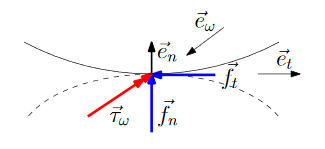
The intuition is that there is a contact area with a certain pressure distribution in normal and a stress distribution in tangential direction and that the response characteristics provides an approximation of the resultant contact normal force $\vec{f}_n$, resultant tangential force $\vec{f}_t$, and resultant contact torque $\vec{\tau}.$ The MPR algorithm calculates an approximation of the contact point, of the signed distance $\delta$ and of a unit vector $\vec{e}_n$ that is orthogonal to the contacting surfaces. When penetration occurs, $\delta \ge 0$, and the contact response is computed from the elastic contact materials of the two objects in the following way, for more details see [4] (the contact force law in normal direction is based on [1], [3], the remaining force law on [2] with some extensions and corrections):
\[\begin{align} f_n &= k_{red} \max\left(0, c_{res} \cdot c_{geo} \cdot \delta^{n_{geo}} \cdot (1 + d \cdot \dot{\delta}) \right) \\ \vec{f}_n &= f_n \cdot \vec{e}_n \\ \vec{f}_t &= -\mu_{k} \cdot f_n \cdot \vec{e}_{t,reg} \\ \vec{\tau} &= -\mu_{r} \cdot \mu_{r,geo} \cdot f_n \cdot \vec{e}_{\omega,reg} \end{align}\]
where
- $\vec{e}_n$: Unit vector perpendicular to the surface of object 1 at the contact point, pointing outwards.
- $\vec{e}_{t,reg}$: Regularized unit vector in direction of the tangential relative velocity (see below).
- $\vec{e}_{\omega,reg}$: Regularized unit vector in direction of the relative angular velocity (see below).
- $f_n$: Value of normal contact force in direction of $\vec{e}_n$ acting on object 2 ($f_n \ge 0$).
- $\vec{f}_n$: Vector of normal contact force acting on object 2.
- $\vec{f}_t$: Vector of sliding friction force acting on object 2 in opposite direction of the movement in the tangential plane of the contact.
- $\vec{\tau}$: Vector of rolling resistance torque acting on object 2, in opposite direction to the relative angular velocity between the two contacting objects.
- $\delta$: Signed distance between object 1 and 2 in normal direction $\vec{e}_n$. $\delta > 0$ if objects are penetrating each other.
- $\dot{\delta}$: Signed relative velocity between object 1 and 2 in normal direction $\vec{e}_n$.
- $c_{res}$: Resultant elastic material constant in normal direction. This constant is computed from the constants $c_1, c_2$ of the two contacting objects 1 and 2 as $c_{res} = 1/\left( 1/c_1 + 1/c_2 \right)$. $c_i$ is computed from the material properties as $c_i = E_i/(1 - \nu_i^2)$ where $E_i$ is Young's modules and $\nu_i$ is Poisson's ratio of object i.
- $c_{geo}$: Factor in $f_n$ that is determined from the geometries of the two objects (see below).
- $n_{geo}$: Exponent in $f_n$ that is determined from the geometries of the two objects (see below).
- $d(cor_{cur},\dot{\delta}^-)$: Damping coefficient in normal direction as a function of $cor_{cur}$ and $\dot{\delta}^-$ (see below).
- $cor_{cur}$: Current coefficient of restitution between objects 1 and 2, see below.
- $\dot{\delta}^-$: Value of $\dot{\delta}$ when contact starts ($\dot{\delta}^- \ge 0$).
- $\mu_k$: Kinetic/sliding friction force coefficient between objects 1 and 2.
- $\mu_r$: Rotational rolling resistance torque coefficient between objects 1 and 2.
- $\mu_{r,geo}$: Factor in $\vec{\tau}$ that is determined from the geometries of the two objects (see below).
- $k_{red}$: Elastic contact reduction factor.
The $\max(..)$ operator in equation (1) is conceptually provided, in order to guarantee that $f_n$ is always a compressive and never a pulling force because this would be unphysical. In the actual implementation no $max(..)$ function is used, because an event is triggered when $\delta$ drops below zero (so no penetration anymore) and after the event no force/torque is applied anymore (meaning that $f_n$ is only evaluated for about $\delta > - 10^{-19} .. - 10^{-24} ~m$ (this depends on the contact situation and the contact materials)).
In special cases (for example sphere rolling on a plane), the rotational coefficient of friction $\mu_{r,res}$ can be interpreted as rolling resistance coefficient.
Coefficients $c_{geo}, n_{geo}, \mu_{r,geo}$ depend on the geometries of the objects that are in contact. The coefficients are computed approximately based on the contact theory of Hertz [5], [6]: Here, it is assumed that each of the contacting surfaces can be described by a quadratic polynomial in two variables that is basically defined by its principal curvatures along two perpendicular directions at the point of contact. A characteristic feature is that the contact volume increases nonlinearly with the penetration depth, so $n_{geo} > 1$ (provided the two contacting surfaces are not completely flat), and therefore the normal contact force changes nonlinearly with the penetration depth. In the general case, elliptical integrals have to be solved, as well as a nonlinear algebraic equation system to compute the normal contact force as function of the penetration depth and the principal curvatures at the contact point. An approximate analytical model is proposed in [7].
In order that a numerical integration algorithm with step-size control works reasonably, the contact force needs to be continuous and continuously differentiable with respect to the penetration depth. This in turn means that the principal curvatures of the contacting surfaces should also be continuous and continuously differentiable, which is usually not the case (besides exceptional cases, such as a Sphere or an Ellipsoid).
Since the determination of the principal curvatures of shapes is in general complicated and the shapes have often areas with discontinuous curvatures, only a very rough approximation is used in Modia3D: The contact area of a shape is approximated by a quadratic polynomial with constant mean principal curvature in all directions and on all points on the shape. In other words, a sphere with constant sphere radius $r_{contact}$ is associated with every shape that is used to compute coefficients $c_{geo}, n_{geo}, \mu_{r,geo}$. A default value for $r_{contact}$ is determined based on the available data of the shape (see Shapes). If a user specific contactSphereRadius is defined in Solid, it is taken instead of the default value.
The default $r_{contact}$ values for each shape are:
| Shape | $r_{contact}$ | isFlat |
|---|---|---|
| Sphere | diameter/2 | false |
| Ellipsoid | min(lengthX, lengthY, lengthZ)/2 | false |
| Box | min(lengthX, lengthY, lengthZ)/2 | true |
| Cylinder | min(diameter, length)/2 | false |
| Cone | (diameter + topDiameter)/4 | false |
| Capsule | diameter/2 | false |
| Beam | min(length, width, thickness)/2 | true |
| FileMesh | shortestEdge/2 | false |
For flat shapes, Box and Beam, $r_{contact}$ is only used, if two flat shapes are in contact with each other ($r_i$ is the contact sphere radius $r_{contact}$ of shape $i$):
| isFlat | isFlat | $\mu_{r,geo}$ |
|---|---|---|
| false | false | $\dfrac{r_1 r_2}{r_1 + r_2}$ |
| false | true | $r_1$ |
| true | false | $r_2$ |
| true | true | $\dfrac{r_1 r_2}{r_1 + r_2}$ |
The factors $n_{geo}, c_{geo}$ in the definition of $f_n$ are computed with the equations for Hertz pressure:
\[\begin{align} n_{geo} &= 1.5 \\ c_{geo} &= \dfrac{4}{3} \sqrt{\mu_{r,geo}} \end{align}\]
Regularized unit vectors
The unit vectors $\vec{e}_t, \vec{e}_{\omega}$ are undefined if the relative velocity and/or the relative angular velocity vanish. They are therefore approximately calculated using utility function $reg(v_{abs}, v_{small})$. This function returns $v_{abs}$ if $v_{abs} \ge v_{small}$ and otherwise returns a third order polynomial with a minimum of $v_{small}/3$ at $v_{abs}=0$ and smooth first and second derivatives at $v_{abs} = v_{small}$):
\[reg(v_{abs}, v_{small}) = \text{if}~ v_{abs} \ge v_{small} ~\text{then}~ v_{abs} ~\text{else}~ \frac{v_{abs}^2}{v_{small}} \left( 1 - \frac{v_{abs}}{3v_{small}} \right) + \frac{v_{small}}{3}\]
Example for $v_{small} = 0.1$:

With $\vec{v}_i$ the absolute velocity of the contact point of object $i$, and $\vec{\omega}_i$ the absolute angular velocity of object $i$, the regularized unit vectors are calculated with function $reg(...)$ in the following way:
\[\begin{align} \vec{e}_{t,reg} =& \frac{\vec{v}_{rel,t}}{reg(|\vec{v}_{rel,t}|, v_{small})}; \quad \vec{v}_{rel} = \vec{v}_2 - \vec{v}_1; \; \vec{v}_{rel,t} = \vec{v}_{rel} - (\vec{v}_{rel} \cdot \vec{e}_n) \vec{e}_n \\ \vec{e}_{\omega,reg} =& \frac{\vec{\omega}_{rel}}{reg(|\vec{\omega}_{rel}|,\omega_{small})}; \quad \vec{\omega}_{rel} = \vec{\omega}_2 - \vec{\omega}_1 \end{align}\]
The effect is that the absolute value of a regularized unit vector is approximated by the following smooth characteristics (and therefore the corresponding friction force and contact torque have a similar characteristic)

Damping coefficient
There are several proposal to compute the damping coefficient as a function of the coefficient of restitution $cor$ and the velocity when contact starts $\dot{\delta}^-$. For a comparision of the different formulations see [1], [3].
Whenever the coefficient of restitution $cor > 0$, then an object 2 jumping on an object 1 will mathematically never come to rest, although this is unphysical. To fix this, the value of a coefficient of restitution is set to zero at contact start when the normal velocity at this time instant is smaller as $v_{small}$:
\[cor_{cur} = \text{if}~ |\dot{\delta}^-| > v_{small} ~\text{then}~ cor ~\text{else}~ 0\]
The damping coefficient $d$ is basically computed with the formulation from [1] because a response calculation with impulses gives similar results for some experiments as shown in [3]. However, (a) instead of $cor$, the current coefficient of restitution $cor_{cur}$ is used and (b) the damping coefficient is limited to $d_{max}$ (this parameter is set via maximumContactDamping in object Scene and has a default value of $2000 ~Ns/m$) to avoid an unphysical strong creeping effect for collisions with small $cor_{cur}$ values:
\[d(cor_{cur},\dot{\delta}^-) = \min(d_{max}, \frac{8(1-cor_{cur})}{5 \cdot cor_{cur} \cdot \dot{\delta}^-})\]
Note, if $cor_{cur} = 0$, then $d = min(d_{max}, 8/0) = d_{max}$.
Examples of this characteristics are shown in the next figure:

In the next figure the simulation of a bouncing ball is shown where the response calculation is performed (a) with an impulse and (b) with the compliant force law above. In both cases the coefficient of restitution $cor$ is zero when $|\dot{\delta}^-| < 0.01$. As can be seen, both formulations lead to similar responses:

Literature
- 1Paulo Flores, Margarida Machado, Miguel Silva, Jorge Martins (2011): On the continuous contact force models for soft materials in multibody dynamics. Multibody System Dynamics, Springer Verlag, Vol. 25, pp. 357-375. 10.1007/s11044-010-9237-4.
- 2Martin Otter, Hilding Elmqvist, José Díaz López (2005): Collision Handling for the Modelica MultiBody Library. Proceedings of the 4th International Modelica Conference 2005, Gerhard Schmitz (Ed.), pages 45-53.
- 3Luka Skrinjar, Janko Slavic, Miha Boltezar (2018): A review of continuous contact-force models in multibody dynamics. International Journal of Mechanical Sciences, Volume 145, Sept., pages 171-187.
- 4Andrea Neumayr, Martin Otter (2019): Collision Handling with Elastic Response Calculation and Zero-Crossing Functions. Proceedings of the 9th International Workshop on Equation-Based Object-Oriented Modeling Languages and Tools. EOOLT’19. ACM, pp. 57–65.
- 5Hertz H. (1881): Über die Berührung fester elastischer Körper. Journal für die reine und angewandte Mathematik 92, S. 156-171.
- 6Johnson K.L. (1985): Contact Mechanics. Cambridge University Press.
- 7Antoine J-F., Visa C., and Sauvey C. (2006): Approximate Analytical Model for Hertzian Elliptical Contact Problems. Transactions of the ASME, Vol. 128. pp. 660-664.