3 Simulation
A particular model is instantiated, simulated and results plotted with the commands:
using Modia
@usingModiaPlot

filter = @instantiateModel(Filter)
simulate!(filter, stopTime=10.0)
plot(filter, "y", figure=1)
3.1 Instantiating
The @instantiateModel macro takes additional arguments:
modelInstance = @instantiateModel(model; FloatType = Float64, aliasReduction=true, unitless=false,
        evaluateParameters=false, log=false, logModel=false, logDetails=false, logStateSelection=false,
        logCode=false,logExecution=logExecution, logCalculations=logCalculations, logTiming=false)
The macro performs structural and symbolic transformations, generates a function for calculation of derivatives suitable for use with DifferentialEquations.jl and returns InstantiatedModel that can be used in other functions, for example to simulate or plot results. Explanation of the arguments:
model: model (declarations and equations)FloatType: Variable type for floating point numbers, for example: Float64, Measurements{Float64}, StaticParticles{Float64,100}, Particles{Float64,2000}aliasReduction: Perform alias elimination and remove singularitiesunitless: Remove units (useful while debugging models and needed for MonteCarloMeasurements)evaluateParameters: Use evaluated parameters in the generated code.log: Log the different phases of translationlogModel: Log the variables and equations of the modellogDetails: Log internal data during the different phases of translationlogStateSelection: Log details during state selectionlogCode: Log the generated codelogExecution: Log the execution of the generated code (useful for timing compilation)logCalculations: Log the calculations of the generated code (useful for finding unit bugs)logTiming: Log timing of different phasesreturn modelInstance prepared for simulation
3.2 Simulating
The simulate! function performs one simulation with DifferentialEquations.jl using by default integrator Sundials.CVODE_BDF(), provided instantiatedModel has FloatType = Float64. Otherwise, a default algorithm will be chosen from DifferentialEquations (for details see https://arxiv.org/pdf/1807.06430, Figure 3). The reason to choose CVODE_BDF as default integrator is that it is a very robust integrator and also usually very efficient for larger models, provided there are no undamped vibrations. It is also possible to specify the integrator as second argument of simulate!:
using Modia
@usingModiaPlot

filter = @instantiateModel(Filter)
sol = simulate!(filter, Tsit5(), stopTime=10.0, merge=Map(T=0.5, x=0.8))
plot(filter, ["y", "x"], figure=1)
Integrator DifferentialEquations.Tsit5 is an adaptive Runge-Kutta method of order 5/4 from Tsitouras. There are > 100 ODE integrators provided. For details, see here.
Parameters and init/start values can be changed with the merge keyword. The effect is the same, as if the filter would have been instantiated with:
filter = @instantiateModel(Filter | Map(T=0.5, x=Var(init=0.8))Note, with the merge keyword in simulate!, init/start values are directly given as a value (x = 0.8) and are not defined with Var(..).
Function simulate! returns sol which is the value that is returned by function DifferentialEquations.solve. Functions of DifferentialEquations that operate on this return argument can therefore also be used on the return argument sol of simulate!.
3.4 Plotting
A short overview of the most important plot commands is given in section Results and Plotting
3.5 State selection (DAEs)
Modia has a sophisticated symbolic engine to transform high index DAEs (Differential Algebraic Equations) automatically to ODEs (Ordinary Differential Equations in state space form). During the transformation, equations might be analytically differentiated and code might be generated to solve linear equation systems numerically during simulation. The current engine cannot transform a DAE to ODE form, if the DAE contains nonlinear algebraic equations. There is an (internal) prototype available to transform nearly any DAE system to a special index 1 DAE system that can be solved with standard DAE integrators. After a clean-up phase, this engine will be made publicly available at some time in the future. Some of the algorithms used in Modia are described in Otter and Elmqvist (2017). Some algorithms are not yet published.
Usually, the symbolic engine is only visible to the modeler, when the model has errors, or when the number of ODE states is less than the number of DAE states. The latter case is discussed in this section.
The following object diagram shows two rotational inertias that are connected by an ideal gear. One inertia is actuated with a sinusoidal torque:
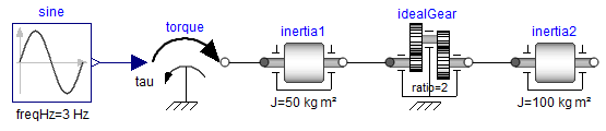
In order to most easily understand the issues, this model is provided in a compact, "flattened" form:
TwoInertiasAndIdealGearTooManyInits = Model(
    J1    = 50,
    J2    = 100,
    ratio = 2,
    f     = 3, # Hz

    phi1 = Var(init = 0.0), # Absolute angle of inertia1
    w1   = Var(init = 0.0), # Absolute angular velocity of inertia1
    phi2 = Var(init = 0.0), # Absolute angle of inertia2
    w2   = Var(init = 0.0), # Absolute angular velocity of inertia2

    equations = :[
        tau = 2.0*sin(2*3.14*f*time/u"s")

        # inertia1
        w1 = der(phi1)
        J1*der(w1) = tau - tau1

        # ideal gear
        phi1 = ratio*phi2
        ratio*tau1 = tau2

        # inertia2
        w2 = der(phi2)
        J2*der(w2) = tau2
    ]
)

drive1 = @instantiateModel(TwoInertiasAndIdealGearTooManyInits)
simulate!(drive1, Tsit5(), stopTime = 1.0, logStates=true)
plot(drive1, [("phi1", "phi2"), ("w1", "w2")])
The option logStates=true results in the following output:
... Simulate model TwoInertiasAndIdealGearTooManyInits

│ # │ state  │ init │ unit │ nominal │
├───┼────────┼──────┼──────┼─────────┤
│ 1 │ phi2   │ 0.0  │      │ NaN     │
│ 2 │ w2     │ 0.0  │      │ NaN     │
This model translates and simulates without problems.
Changing the init-value of w2 to 1.0 and re-simulating:
simulate!(drive1, Tsit5(), stopTime = 1.0, logStates=true, merge = Map(w2=1.0))results in the following error:
... Simulate model TwoInertiasAndIdealGearTooManyInits

│ # │ state │ init │ unit │ nominal │
├───┼───────┼──────┼──────┼─────────┤
│ 1 │ phi2  │ 0.0  │      │ NaN     │
│ 2 │ w2    │ 1.0  │      │ NaN     │


Error from simulate!:
The following variables are explicitly solved for, have init-values defined
and after initialization the init-values are not respected
(remove the init-values in the model or change them to start-values):

│ # │ name │ beforeInit │ afterInit │
├───┼──────┼────────────┼───────────┤
│ 1 │ w1   │ 0.0        │ 2.0       │
The issue is the following:
Every variable that is used in the der operator is a potential ODE state. When an init value is defined for such a variable, then Modia either utilizes this initial condition (so the variable has this value after initialization), or an error is triggered, as in the example above.
The model contains the equation:
phi1 = ratio*phi2So the potential ODE states phi1 and phi2 are constrained, and only one of them can be selected as ODE state, and the other variable is computed from this equation. Since parameter ratio can be changed before simulation is started, it can be changed also to a value of ratio = 0. Therefore, only when phi2 is selected as ODE state, phi1 can be uniquely computed from this equation. If phi1 would be selected as ODE state, then a division by zero would occur, if ratio = 0, since phi2 = phi1/ratio. For this reason, Modia selects phi2 as ODE state. This means the init value of phi1 has no effect. This is uncritical, as long as initialization computes this init value from the constraint equation above, as done in the example above.
When differentiating the equation above:
der(phi1) = ratio*der(phi2)  # differentiated constraint equation
       w1 = der(phi1)
       w2 = der(phi2)
it becomes obvious, that there is also a hidden constraint equation for the potential ODE states w1, w2:
w1 = ratio*w2 # hidden constraint equationAgain, Modia selects w2 as ODE state, and ignores the init value of w1. In the second simulation, the init value of w1 (= 0.0) is no longer consistent to the init value of w2 (= 1.0). Therefore, an error occurs.
The remedy is to remove the init values of phi1, w1 from the model:
drive2 = @instantiateModel(TwoInertiasAndIdealGearTooManyInits |
                                Map(phi1 = Var(init=nothing),
                                    w1   = Var(init=nothing)) )
simulate!(drive2, Tsit5(), stopTime = 1.0, logStates=true, merge = Map(w2=1.0))
and simulation is successful!
Modia tries to respect init values during symbolic transformation. In cases as above, this is not possible and the reported issue occurs. In some cases, it might not be obvious, why Modia selects a particular variable as an ODE state. You can get more information by setting logStateSelection=true:
drive1 = @instantiateModel(TwoInertiasAndIdealGearTooManyInits, logStateSelection=true)This results in the following output in the REPL:
Instantiating model TwoInertiasAndIdealGearTooManyInits
  in module: Main.Tutorial
  in file: <..>\Modia\examples\Tutorial.jl:196

=== getSortedAndSolvedAST(...) started for TwoInertiasAndIdealGearTooManyInits.

... Equation set 1.1 ..............................
Equations:
   1: tau = 2.0 * sin((2 * 3.14 * f * time) / u"s")
Unknown variables:
   1: tau
One equation in one unknown variable. Solve the equation:
Julia code:
    tau = 2.0 * sin((2 * 3.14 * _FloatType(_p[:f])::_FloatType * time) / u"s")

... Equation set 2.1 ..............................
Equations:
   4: phi1 = ratio * phi2
Unknown variables:
   7: phi2
   4: phi1
1 equation(s) in 2 unknown variable(s). Tear the system of equations:
    Unknowns with start or init values: phi2, phi1
    Tearing  variables: phi2
    All solved unknowns are dummy states.
Julia code:
    phi1 = _FloatType(_p[:ratio])::_FloatType * phi2

... Equation set 2.2 ..............................
Equations:
   6: w2 = der(phi2)
   8: der(phi1) = ratio * der(phi2)
   2: w1 = der(phi1)
Unknown variables:
   9: w2
  10: der(phi2)
   3: der(phi1)
   2: w1
3 equation(s) in 4 unknown variable(s). Tear the system of equations:
    Unknowns with start or init values: w2, w1
    Tearing  variables: w2
    All solved unknowns are dummy states.
Julia code:
    var"der(phi2)" = w2
    var"der(phi1)" = _FloatType(_p[:ratio])::_FloatType * var"der(phi2)"
    w1 = var"der(phi1)"

... Equation set 2.3 ..............................
Equations:
   5: ratio * tau1 = tau2
   7: J2 * der(w2) = tau2
  10: der(w2) = der(der(phi2))
  11: der(der(phi1)) = ratio * der(der(phi2))
   9: der(w1) = der(der(phi1))
   3: J1 * der(w1) = tau - tau1
Unknown variables:
   8: tau2
  11: der(w2)
  13: der(der(phi2))
  12: der(der(phi1))
   5: der(w1)
   6: tau1
6 equation(s) in 6 unknown variable(s). Tear the system of equations:
    Tearing  variables: der(w2)
    Residual equations:
       7: J2 * der(w2) = tau2
    All unknowns are solved.
Teared equation system is linear. Solve system with hasConstantCoefficients = false.
code = quote
    local var"der(w2)", var"der(der(phi2))", var"der(der(phi1))", var"der(w1)", tau1, tau2
    _leq_mode = initLinearEquationsIteration!(_m, 1)
     ModiaBase.TimerOutputs.@timeit _m.timer "ModiaBase LinearEquationsIteration!" while ModiaBase.LinearEquationsIteration!(_leq_mode, _m.isInitial, _m.solve_leq, _m.storeResult, _m.time, _m.timer)
            var"der(w2)" = _leq_mode.x[1] * u"s^-1"
            var"der(der(phi2))" = var"der(w2)"
            var"der(der(phi1))" = _FloatType(_p[:ratio])::_FloatType * var"der(der(phi2))"
            var"der(w1)" = var"der(der(phi1))"
            tau1 = -((_FloatType(_p[:J1])::_FloatType * var"der(w1)" - tau))
            tau2 = _FloatType(_p[:ratio])::_FloatType * tau1
            ModiaBase.appendVariable!(_leq_mode.residuals, Modia.Unitful.ustrip.(tau2) .- Modia.Unitful.ustrip.(_FloatType(_p[:J2])::_FloatType * var"der(w2)"))
        end
    _leq_mode = nothing
end
Sort equations (BLT on all equations under the assumption that the ODE states are known).

Information message from getSortedAndSolvedAST for model TwoInertiasAndIdealGearTooManyInits:
The following variables are iteration variables but have no start/init values defined.
If units are used in the model, start/init values with correct units should be defined
to avoid unit errors during compilation.
Involved variables:
    der(w2)


Warning message from getSortedAndSolvedAST for model TwoInertiasAndIdealGearTooManyInits:
The following variables have an 'init' initialization and are explicitly solved for.
Therefore, the 'init' values have no effect, but must exactly match the values,
computed during initialization. Otherwise this gives a run-time error.
It is adviced to use 'start' initialization or remove initialization for these variables.
Involved variables:
    phi1
    w1