Functions
Instantiation
Modia.@instantiateModel — MacromodelInstance = @instantiateModel(model; FloatType = Float64, aliasReduction=true, unitless=false,
evaluateParameters=false, saveCodeOnFile="", log=false, logModel=false, logDetails=false, logStateSelection=false,
logCode=false,logExecution=logExecution, logCalculations=logCalculations, logTiming=false, logFile=true)Instantiates a model, i.e. performs structural and symbolic transformations and generates a function for calculation of derivatives suitable for simulation.
model: model (declarations and equations)FloatType: Variable type for floating point numbers, for example: Float64, Measurement{Float64}, StaticParticles{Float64,100}, Particles{Float64,2000}aliasReduction: Perform alias elimination and remove singularitiesunitless: Remove units (useful while debugging models and needed for MonteCarloMeasurements)evaluateParameters: Use evaluated parameters in the generated code.saveCodeOnFile: If non-empty string, save generated code in file with namesaveCodeOnFile.log: Log the different phases of translationlogModel: Log the variables and equations of the modellogDetails: Log internal data during the different phases of translationlogStateSelection: Log details during state selectionlogCode: Log the generated codelogExecution: Log the execution of the generated code (useful for timing compilation)logCalculations: Log the calculations of the generated code (useful for finding unit bugs)logTiming: Log timing of different phaseslogFile: Log file and line number where @instantiatedModel is calledreturn modelInstance prepared for simulation
Modia.instantiateModel — FunctionSee documentation of macro [@instantiateModel]
Simulation
Modia.simulate! — Functionsolution = simulate!(instantiatedModel [, algorithm];
merge = missing, # change parameter/init/start values
tolerance = 1e-6, # relative tolerance
startTime = 0.0,
stopTime = 0.0, # stopTime >= startTime required
interval = missing, # = (stopTime-startTime)/500
interp_points = 0,
dtmax = missing, # = 100*interval
adaptive = true,
nlinearMinForDAE = 10,
log = false,
logStates = false,
logEvents = false,
logProgress = false,
logTiming = false,
logParameters = false,
logEvaluatedParameters = false,
requiredFinalStates = missing
requiredFinalStates_rtol = 1e-3,
requiredFinalStates_atol = 0.0,
useRecursiveFactorizationUptoSize = 0)Simulate instantiatedModel::InstantiatedModel with algorithm (= alg of ODE Solvers of DifferentialEquations.jl or DAE Solvers of DifferentialEquations.jl).
If the algorithm argument is missing, algorithm=Sundials.CVODE_BDF() is used, provided instantiatedModel has FloatType = Float64. Otherwise, a default algorithm will be chosen from DifferentialEquations (for details see https://arxiv.org/pdf/1807.06430, Figure 3). The symbols CVODE_BDF and IDA are exported from Modia, so that simulate!(instantiatedModel, CVODE_BDF(), ...) and simulate!(instantiatedModel, IDA(), ...) can be used (instead of import Sundials; simulate!(instantiatedModel, Sundials.xxx(), ...)).
The simulation results are stored in instantiatedModel and can be plotted with plot(instantiatedModel, ...). The result values can be retrieved with getValues(..) for Var(..) and getValue(..) for Par(..). showInfo(instantiatedModel) prints information about the signals in the result. For more details, see sections Parameters/Init/Start, Results and Plotting.
The return argument solution is the return argument from DifferentialEquations.solve(..) and therefore all post-processing functionality from DifferentialEqautions.jl can be used. Especially,
- solution.t[i] # time-instant at storage point i (solution.t[end] = stopTime)
- solution.u[i] # states at storage point i
A simulation run can be aborted with <CTRL> C (SIGINT), provided using PyPlot or import PyPlot was not called before (the signals in Python module matplotlib.pyplot intervene with Julias signals, see PyPlot.jl issue 305).
Optional ArgumentsS
merge: Define parameters and init/start values that shall be merged with the previous values stored inmodel, before simulation is started. If, say, an init valuephi = Var(init=1.0)is defined in the model, a different init value can be provided withmerge = Map(phi=2.0).tolerance: Relative tolerance.startTime: Start time. If value is without unit, it is assumed to have unit [s].stopTime: Stop time. If value is without unit, it is assumed to have unit [s].interval: Interval to store result. Ifinterval=missing, it is internally selected as (stopTime-startTime)/500. If value is without unit, it is assumed to have unit [s].interp_points: If crossing functions defined, number of additional interpolation points in one step.dtmax: Maximum step size. Ifdtmax==missing, it is internally set to100*interval.adaptive: = true, if thealgorithmshould use step-size control (if available). = false, if thealgorithmshould use a fixed step-size ofinterval(if available).nlinearMinForDAE: Ifalgorithmis a DAE integrator (e.g.IDA()) and the size of a linear equation system is>= nlinearMinForDAEand the iteration variables of this equation system are a subset of the DAE state derivatives, then during continuous integration (but not at events, including initialization) this equation system is not locally solved but is solved via the DAE integrator. Typically, for large linear equation systems, simulation efficiency is considerably improved in such a case.flog: = true, to log the simulation.logStates: = true, to log the states, its init/start values and its units.logEvents: = true, to log events.logProgress= true, to printout current simulation time every 5s.logTiming: = true, to log the timing withinstantiatedModel.timerwhich is an instance of TimerOutputs.TimerOutput. A user function can include its timing via
TimerOutputs.@timeit instantiatedModel.timer "My Timing" <statement>.logParameters: = true, to log parameters and init/start values defined in model.logEvaluatedParameters: = true, to log the evaluated parameter and init/start values that are used for initialization and during simulation.requiredFinalStates: is notmissing: Test with@testwhether the ODE state vector at the final time instant is in agreement to vectorrequiredFinalStateswith respect to tolerancesrequiredFinalStates_rtol, requiredFinalStates_atol. If this is not the case, print the final state vector (so that it can be included with copy-and-paste in the simulate!(..) call). If you checked that the result of the simulation is correct, userequiredFinalStates = []to get a printout of the required final states and then copy it in your test.requiredFinalStates_rtol: Relative tolerance used forrequiredFinalStates.requiredFinalStates_atol: Absolute tolerance used forrequiredFinalStates(see atol in?isapprox)useRecursiveFactorizationUptoSize: = 0: Linear equation systems A*v=b are solved withRecursiveFactorization.jlinstead of the defaultlu!(..)andldiv!(..), iflength(v) <= useRecursiveFactorizationUptoSize. According toRecursiveFactorization.jldocu, it is faster aslu!(..)with OpenBLAS, forlength(v) <= 500(typically, more as a factor of two). Since there had been some cases wherelu!(..)!was successful, butRecursiveFactorization.jlfailed due to a singular system, the default is to uselu!(..)!.
Examples
using Modia
@usingModiaPlot

# Define model
inputSignal(t) = sin(t)

FirstOrder = Model(
    T = 0.2,
    x = Var(init=0.3),
    equations = :[u = inputSignal(time/u"s"),
                  T * der(x) + x = u,
                  y = 2*x]
)

# Modify parameters and initial values of model
FirstOrder2 = FirstOrder | Map(T = 0.4, x = Var(init=0.6))

# Instantiate model
firstOrder = @instantiateModel(FirstOrder2, logCode=true)


# Simulate with automatically selected algorithm (Sundials.CVODE_BDF())
# and modified parameter and initial values
simulate!(firstOrder, stopTime = 1.0, merge = Map(T = 0.6, x = 0.9), logEvaluatedParameters=true)

# Plot variables "x", "u" in diagram 1, "der(x)" in diagram 2, both diagrams in figure 3
plot(firstOrder, [("x","u"), "der(x)"], figure=3)

# Retrieve "time" and "u" values:
usig = getPlotSignal(firstOrder, "x")
       # usig.xsig      : time vector
       # usig.xsigLegend: legend for time vector
       # usig.ysig      : "x" vector
       # usig.ysigLegend: legend for "x" vector
       # usig.ysigType  : ModiaResult.Continuous or ModiaResult.Clocked

# Simulate with Runge-Kutta 5/4 with step-size control
simulate!(firstOrder, Tsit5(), stopTime = 1.0)

# Simulate with Runge-Kutta 4 with fixed step size
simulate!(firstOrder, RK4(), stopTime = 1.0, adaptive=false)

# Simulate with algorithm that switches between
# Verners Runge-Kutta 6/5 algorithm if non-stiff region and
# Rosenbrock 4 (= A-stable method) if stiff region with step-size control
simulate!(firstOrder, AutoVern6(Rodas4()), stopTime = 1.0)Linearization
Modia.linearize! — Function(A, finalStates) = linearize!(instantiatedModel [, algorithm];
stopTime = 0.0,
analytic = false,
<all other keyword arguments of simulate!>)Simulate until stopTime and linearize instantiatedModel at finalStates. The names of the state vector can be inquired by get_xNames(instantiatedModel).
By default, linearization is performed numerically with a central finite difference approximation using package FiniteDiff. When setting analytic = true, linearization is preformed analytically with package ForwardDiff, so is computed by symbolically differentiating the model. ForwardDiff might not be compatible with some floating point types, such as Measurements and Julia triggers an error that some overloaded operations are ambiguous. So analytic=true will not work in such cases.
Analytic linearization returns matrix A in full precision whereas numeric linearization returns A in reduced precision (if FloatType = Float64, analytic linearization results in about 15 correct digits and numeric linearization in about 10 correct digits in the result). You can improve this situation, by using a larger FloatType for instantiatedModel, in case this is critical (see example below).
Output arguments
A::Matrix: Matrix A of the linear ODE: $\Delta \dot{x} = A*\Delta x$.finalStates::Vector: Linearization point.
Example
using Modia
using DoubleFloats
using Measurements

FirstOrder = Model(
    T = 0.4 ± 0.04,
    x = Var(init = 0.9 ± 0.09),
    equations = :[u = inputSignal(time/u"s"),
                  T * der(x) + x = u]
)

firstOrder1 = @instantiateModel(FirstOrder, FloatType = Measurement{Float64})

# Standard precision
(A1, finalStates1) = linearize!(firstOrder1)

# Higher precision
firstOrder2 = InstantiatedModel{Measurement{Double64}}(firstOrder1)
(A2, finalStates2) = linearize!(firstOrder2)

# Show results with 15 digits (default print with Measurements shows 3 digits)
println(IOContext(stdout, :error_digits=>15), "A1 = ", A1)
println(IOContext(stdout, :error_digits=>15), "A2 = ", A2)Parameters/Init/Start
The following functions are provided to inquire values of parameters and of init/start values before and after evaluation:
| Functions | Description |
|---|---|
hasParameter | Return true, if a parameter/init/start name is known |
getParameter | Return value of a parameter/init/start name |
getEvaluatedParameter | Return value of an evaluated parameter/init/start name |
getLastValue | Return last available value of a variable name |
showParameters | Print the parameters and the init/start values |
showEvaluatedParameters | Print the evaluated parameters and init/start values |
Modia.hasParameter — FunctionhasParameter(instantiatedModel, name::AbstractString)Return true if parameter name (for example name = "a.b.c") is defined in the instantiateModel.
Modia.getParameter — FunctiongetParameter(instantiatedModel, name::AbstractString)Return the value of parameter or init/start value name (for example name = "a.b.c"). If name is not known, missing is returned.
Modia.getEvaluatedParameter — FunctiongetEvaluatedParameter(instantiatedModel, name::AbstractString)Return the value of evaluated parameter or init/start value name (for example name = "a.b.c"). If name is not known, missing is returned.
Modia.getLastValue — FunctiongetLastValue(model::InstantiatedModel, name::String; unit=true)Return the last stored value of variable name from model. If unit=true return the value with its unit, otherwise with stripped unit.
If name is not known or no result values yet available, an info message is printed and the function returns nothing.
name can be a time-varying variable or a parameter.
Modia.showParameters — FunctionshowParameters(instantiatedModel)Print the parameters and the init/start values.
Modia.showEvaluatedParameters — FunctionshowEvaluatedParameters(instantiatedModel)Print the evaluated parameters and the evaluated init/start values.
Results and Plotting
The simulation result of a model instantiatedModel are provided as a signal table, see SignalTables.jl.
Therefore, all signal table functions can be used on a simulated model
To activate the defined plot package, use
Alternatively, usingPlotPackage (from Modia reexported macro of SignalTables) can be used, but then package SignalTables must be in your current environment.
Example:
using Modia

FirstOrder = Model(
    T = 0.2u"s",
    x = Var(init=0.3),
    equations = :[u = sin(time/u"s")
                  T * der(x) + x = u
                  y = 2*x]
)
simulate!(firstOrder, stopTime=10)
showInfo(firstOrder)    # list info about the result
t = getValues(firstOrder, "time")
y = getValues(firstOrder, "y")      # use any plot program: plot(t,y)

# Write result on file
writeSignalTable("firstOrder.json", firstOrder, indent=2, log=true)
See the generated json-file.
For plotting, a plot package must be installed, e.g.,
julia> ]add SignalTablesInterface_PyPlot        # if plotting with PyPlot desired
        add SignalTablesInterface_GLMakie       # if plotting with GLMakie desired
        add SignalTablesInterface_WGLMakie      # if plotting with WGLMakie desired
        add SignalTablesInterface_CairoMakie    # if plotting with CairoMakie desired
In a model, the desired plot package is defined with:
using Modia
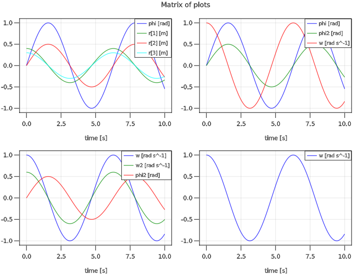
usePlotPackage("PyPlot") # or ENV["SignalTablesPlotPackage"] = "PyPlot"A Modia variable a.b.c is identified by a String key "a.b.c". The legends/labels of the plots are automatically constructed by the names and units of the variables. Example:
using Modia
@usingModiaPlot   # execute `using SignalTablesInterface_XXX` or
                  # execute `using Modia.SignalTables.SilentNoPlot`

instantiatedModel = @instantiateModel(...)
simulate!(instantiatedModel, ...)
plot(instantiatedModel,
     [ ("phi", "r")        ("phi", "phi2", "w");
       ("w", "w2", "phi2") "w"                ],
     heading="Matrix of plots")
generates the following plot:
Modia.@usingModiaPlot — Macro@usingModiaPlot()Execute using XXX, where XXX is the Plot package that was activated with usePlotPackage(plotPackage). So this is similar to @usingPlotPackage (from SignalTables, that is reexported from Modia).
There is, however, a difference when XXX = "SilentNoPlot":
- @usingPlotPackage() executes
using SignalTables.SilentNoPlotand therefore requires that packageSignalTablesis available in your environment. - @usingModiaPlot() executes
using Modia.SignalTables.SilentNoPlotand therefore requires that packageModiais available in your environment.
Therefore, when working with Modia it is better to use @usingModiaPlot().
PathPlanning
There are some pre-defined functions to define reference paths
Modia.PTP_path — Typepath = PTP_path(names; positions, v_max, a_max, startTime=0.0)Generate a new path object to move as fast as possible from positions[i,:] to positions[i+1,:]. The positions[i,:] can be a set of translational positions in [m], that is absolute distances, and/or rotational positions in [rad] that is angles. In robotics such a movement is called PTP (Point-To-Point). The signals are constructed in such a way that it is not possible to move faster, given the maximally allowed velocity v_max[j] and the maximally allowed acceleration a_max[j] for signal names[j] and have a velocity of zero at the given positions.
If there are two or more signals (that is length(names) > 1) then the path is constructed such that all signals are in the same periods in the acceleration, constant velocity and deceleration phase. This means that only one of the signals is at its limits whereas the others are synchronized in such a way that the end point is reached at the same time instant.
For example, this means that the signals have a velocity of zero at positions[1,:], one of the signals is accelerated with its maximally allowed acceleration until one of the signals reaches its maximally allowed velocity. At a proper time instant, one of the signals is decelerated with the negative value of its maximally allowed acceleration, so that all signals reach positions[2,:] with velocity zero.
This element is useful to generate a reference signal for a controller which controls, e.g., a drive train, or to drive a flange according to a given acceleration.
Example
using Modia
@usingModiaPlot

const ptp_path = PTP_path(["angle1", "angle2", "angle3"],
                          positions = [0.0 2.0 3.0;  # angle1=0.0, angle2=2.0, angle3=3.0
                                       0.5 3.0 4.0;
                                       0.8 1.5 0.3;
                                       0.2 1.5 0.8],
                          startTime = 0.1,
                          v_max = 2*ones(3),
                          a_max = 3*ones(3))
angles = zeros(3)
getPosition!(ptp_path, 0.5, angles)   # angles = [0.12, 2.24, 3.24]
path = getPath(ptp_path)
plot(path, ["angle1", "angle2", "angle3"])Modia.pathEndTime — FunctionTend = pathEndTime(path)Given a path::PTP_path return the end time Tend of the path.
Modia.getPosition! — FunctiongetPosition!(path, time, position)Given a path::PTP_path and a time instant time, return the actual position at time time in vector position.
getPosition!(path, time, position, velocity, acceleration)Given a path::PTP_path and a time instant time, return the actual position, velocity and acceleration at time time in vectors position, velocity, acceleration.
Modia.getPosition — Functionpos = getPosition(path, index, time)Given a path::PTP_path, the index of a signal, and a time instant time, return the actual position at time time.
Modia.getIndex — Functionindex = getIndex(path, name)Return the index of name in path or trigger an error, if not present.
Modia.getPath — FunctiongetPath(path;
names=path.names, tend=1.1*path.Tend, ntime=101, onlyPositions=false)Given a path::PTP_path, return a SignalTables.SignalTable with the time series of the path over time up to tend for all ntime time points.