4 Floating Point Types
The types of the floating point numbers in a Modia model can be parameterized with argument FloatType of macro @instantiateModel:
filter = @instantiateModel(Filter; FloatType = Float64)By default, a floating point number has type Float64.
Using another floating point type requires that a DifferentialEquations.jl integrator is used that is implemented in native Julia. An integrator that interfaces an integrator implemented in C (such as CVODE_BDF() the popular Sundials BDF method), cannot be used.
4.1 Lower and higher precision
In principal, any floating point type of Julia (so any type that is derived from AbstractFloat) can be used in the model and the integrators. Examples
| Type | Precision | Package | Usage |
|---|---|---|---|
| Float32 | 7 digits | built-in | Embedded system |
| Float64 | 16 digits | built-in | Offline simulation |
| Double64 | 30 digits | DoubleFloats | High precision needed |
| BigFloat | arbitrary | built-in | Very high precision needed (very slow) |
- The
Float32type might be used to test the execution and numerics of a model that shall later run on an embedded system target (there is no automatic way, yet, to translate a Modia model toC).
Double64is a type that is constructed from two Float64 types. The execution is much faster as the comparable Julia built-in type BigFloat when set to 128 bit precision. TheDouble64type might be used, when simulation withFloat64fails due to numerical reasons (for example the model is very sensitive, or equation systems are close to singularity) or when very stringent relative tolerances are needed, for example relative tolerance = 1e-15 as needed for some space applications.
In the following example, simulation is performed with a Float32 floating point type used for model and integrator and utilizing a Runge-Kutta integrator of order 4 with a fixed step size of 0.01 s:
filter = @instantiateModel(Filter, FloatType = Float32)
simulate!(filter, RK4(), adaptive=false, stopTime=10.0, interval=0.01)
4.2 Uncertainties
Package Measurements provides a floating point type designed for error propagation. A floating point number is defined with a nominal value and an uncertainty:
using Measurements

m1 = 2.1 ± 0.4
m2 = 2*m1           # 4.2 ± 0.8
m3 = m2 - m1        # 2.1 ± 0.4
The statement m1 = 2.1 ± 0.4 defines that m1 has a nominal value of 2.1 with a standard deviation of 0.4. This means that the probability is about 95 % that the value of m1 is in the range 1.3 .. 2.9. Package Measurements computes the error propagation with first-order theory (so this is typically an approximation) by computing the partial derivatives of all variables with respect to all source error definitions and computing the propagated error with this information. The benefit is that the error bounds are typically reasonably propagated and the computation is reasonably fast. The drawback is that it is an approximation and will be not correct, if the uncertainty is too large and/or the signals change too quickly (for example are discontinuous).
The following model defines a simple pendulum where a mass point is attached via a rod and a revolute joint to the environment. It is described by the equations
\[\begin{aligned} \frac{d\varphi}{dt} &= \omega \\ 0 &= m \cdot L^2 \cdot \frac{d\omega}{dt} + d \cdot \omega + m \cdot g \cdot L \cdot sin(\varphi) \end{aligned}\]
where $\varphi$ is the rotation angle, $\omega$ the angular velocity, $m$ the mass, $L$ the rod length, $d$ a damping constant and $g$ the gravity constant. This model can be defined with the commands:
Pendulum = Model(
   L = (0.8±0.1)u"m",
   m = (1.0±0.1)u"kg",
   d = (0.5±0.05)u"N*m*s/rad",
   g = 9.81u"m/s^2",
   phi = Var(init = (pi/2±0.1)*u"rad"),
   w   = Var(init = 0u"rad/s"),
   equations = :[
          w = der(phi)
        0.0 = m*L^2*der(w) + d*w + m*g*L*sin(phi)
   ]
)

pendulum = @instantiateModel(Pendulum, FloatType=Measurements.Measurement{Float64})
simulate!(pendulum, Tsit5(), stopTime = 10.0)
plot(pendulum, "phi")
and simulates the pendulum with uncertain parameter and init values and results in the following plot:
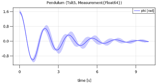
The area around the nominal value of a variable characterizes the standard deviation.
4.3 Monte-Carlo Simulation
The Julia package MonteCarloMeasurements.jl provides calculations with particles. A value can be defined with a distribution of say 2000 values randomly chosen according to a desired distribution and then all calculations are performed with 2000 values at the same time (corresponds to 2000 simulations that are carried out).
In the example below, a modest form of 100 particles (100 simulations) with Uniform distributions of some parameters and init values are defined that correspond roughly to the definition with uncertainties of the previous section (but using uniform instead for normal distributions):
using Modia
using DifferentialEquations
using ModiaPlot
using MonteCarloMeasurements
using Distributions
using Unitful

const nparticles = 100
uniform(vmin,vmax) = StaticParticles(nparticles,Distributions.Uniform(vmin,vmax))

Pendulum = Model(
   L = uniform(0.6, 1.0),
   m = uniform(0.8, 1.2),
   d = uniform(0.4, 0.6),
   g = 9.81,
   phi = Var(init = uniform(pi/2-0.2, pi/2+0.2)),
   w   = Var(init = 0),
   equations = :[
          w = der(phi)
        0.0 = m*L^2*der(w) + d*w + m*g*L*sin(phi)
   ]
)

pendulum = @instantiateModel(Pendulum,FloatType=StaticParticles{Float64,nparticles})
simulate!(pendulum, Tsit5(), stopTime = 10.0)
plot(pendulum, "phi", MonteCarloAsArea=false)
The simulation result is shown in the next figure:
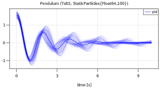
Since plot option MonteCarloAsArea=false is used, all 100 simulations are shown in the plot, together with the mean value of all simulations. The default plot behavior is to show the mean value and the area in which all simulations are contained (this is useful, if there are much more simulations, because GLMakie crashes when there are too many curves in a diagram).
There are currently a few restrictions, in particular units are not yet supported in the combination of Modia and MonteCarloMeasurements, so units are not defined in the model above.