Functions
Instantiation
TinyModia.@instantiateModel — MacromodelInstance = @instantiateModel(model; FloatType = Float64, aliasReduction=true, unitless=false,
log=false, logModel=false, logDetails=false, logStateSelection=false, logCode=false, logExecution=false, logTiming=false)Instantiates a model, i.e. performs structural and symbolic transformations and generates a function for calculation of derivatives suitable for simulation.
model: model (declarations and equations)FloatType: Variable type for floating point numbers, for example: Float64, Measurements{Float64}, StaticParticles{Float64,100}, Particles{Float64,2000}aliasReduction: Perform alias elimination and remove singularitiesunitless: Remove units (useful while debugging models and needed for MonteCarloMeasurements)log: Log the different phases of translationlogModel: Log the variables and equations of the modellogDetails: Log internal data during the different phases of translationlogStateSelection: Log details during state selectionlogCode: Log the generated codelogExecution: Log the execution of the generated code (useful for finding unit bugs)logTiming: Log timing of different phasesreturn modelInstance prepared for simulation
TinyModia.instantiateModel — FunctionSee documentation of macro @instatiateModel
Simulation
TinyModia.simulate! — Functionsimulate!(model [, algorithm]; merge = nothing,
tolerance = 1e-6, startTime = 0.0, stopTime = 1.0, interval = NaN,
adaptive = true, log = true, logParameters = true, logStates = true,
requiredFinalStates = nothing)Simulate model::SimulationModel with algorithm (= alg of ODE Solvers of DifferentialEquations.jl). If the algorithm argument is missing, a default algorithm will be chosen from DifferentialEquations (for details see https://arxiv.org/pdf/1807.06430, Figure 3).
The simulation results stored in model can be plotted with ModiaPlot.plot and the result values can be retrieved with get_result.
Optional Arguments
merge: Define parameters and init/start values that shall be merged with the previous values stored inmodel, before simulation is started.tolerance: Relative tolerance.startTime: Start time. If value is without unit, it is assumed to have unit [s].stopTime: Stop time. If value is without unit, it is assumed to have unit [s].interval: Interval to store result. Ifinterval=NaN, it is internally selected as (stopTime-startTime)/500. If value is without unit, it is assumed to have unit [s].adaptive: = true, if thealgorithmshould use step-size control (if available). = false, if thealgorithmshould use a fixed step-size ofinterval(if available).log: = true, to log the simulation.logParameters: = true, to log the parameter and init/start valueslogStates: = true, to log the states, its init/start values and its units.requiredFinalStates: is notnothing: Check whether the ODE state vector at the final time instant with@testis in agreement to vectorrequiredFinalStateswith respect to some tolerance. If this is not the case, print the final state vector (so that it can be included with copy-and-paste in the simulate!(..) call).
Examples
using ModiaPlot
using DifferentialEquations

# Define model
inputSignal(t) = sin(t)

FirstOrder = Model(
    T = 0.2,
    x = Var(init=0.3),
    equations = :[u = inputSignal(time/u"s"),
                  T * der(x) + x = u,
                  y = 2*x]
)

# Modify parameters and initial values of model
FirstOrder2 = FirstOrder | Map(T = 0.4, x = Var(init=0.6))

# Instantiate model
firstOrder = @instantiateModel(FirstOrder2, logCode=true)


# Simulate with automatically selected algorithm and
# modified parameter and initial values
simulate!(firstOrder, stopTime = 1.0, merge = Map(T = 0.6, x = 0.9), logParameters=true)

# Plot variables "x", "u" in diagram 1, "der(x)" in diagram 2, both diagrams in figure 3
plot(firstOrder, [("x","u"), "der(x)"], figure=3)

# Retrieve "time" and "u" values:
get_result(firstOrder, "time")
get_result(firstOrder, "u")


# Simulate with Runge-Kutta 5/4 with step-size control
simulate!(firstOrder, Tsit5(), stopTime = 1.0)

# Simulate with Runge-Kutta 4 with fixed step size
simulate!(firstOrder, RK4(), stopTime = 1.0, adaptive=false)

# Simulate with algorithm that switches between
# Verners Runge-Kutta 6/5 algorithm if non-stiff region and
# Rosenbrock 4 (= A-stable method) if stiff region with step-size control
simulate!(firstOrder, AutoVern6(Rodas4()), stopTime = 1.0)

# Simulate with Sundials CVODE (BDF method with variable order 1-5) with step-size control
using Sundials
simulate!(firstOrder, CVODE_BDF(), stopTime = 1.0)Plotting
The results of a simulation of a model instantiatedModel can be visualized with function ModiaPlot.plot that produces line plots of the result time series. A variable a.b.c is identified by a String key "a.b.c". The legends/labels of the plots are automatically constructed by the names and units of the variables. Example:
using ModiaPlot
instantiatedModel = @instantiatedModel(...)
simulate!(instantiatedModel, ...)
plot(instantiatedModel,
     [ ("phi", "r")        ("phi", "phi2", "w");
       ("w", "w2", "phi2") "w"                ],
     heading="Matrix of plots")
generates the following plot:
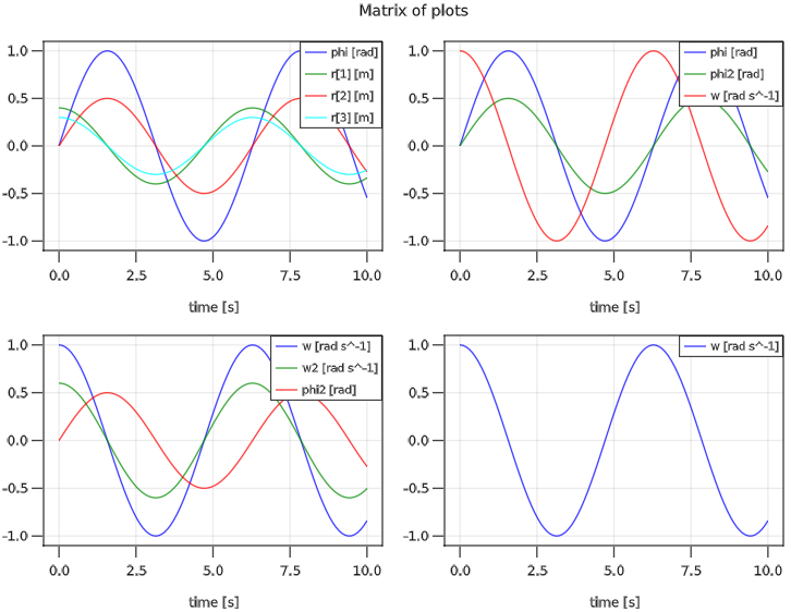
The underlying line plot is generated by GLMakie.
Inquiries
TinyModia.get_result — Functionsignal = get_result(model, name; unit=true)After a successful simulation of model::SimulationModel, return the result for the signal name::String as vector of points together with its unit. The time vector has path name "time". If unit=false, the signal is returned, without unit.
Example
using ModiaBase
using Unitful

include("$(ModiaBase.path)/demos/models/Model_Pendulum.jl")
using  .Model_Pendulum

pendulum = simulationModel(Pendulum)
simulate!(pendulum, stopTime=7.0)

time = get_result(pendulum, "time")  # vector with unit u"s"
phi  = get_result(pendulum, "phi")   # vector with unit u"rad"

import PyPlot
PyPlot.figure(4)   # Change to figure 4 (or create it, if it does not exist)
PyPlot.clf()       # Clear current figure
PyPlot.plot(ustrip(time), ustrip(phi), "b--", label="phi in " * string(unit(phi[1])))
PyPlot.xlabel("time in " * string(unit(time[1])))
PyPlot.legend()TinyModia.get_lastValue — Functionget_lastValue(model::SimulationModel, name::String; unit=true)Return the last stored value of variable name from model. If unit=true return the value with its unit, otherwise with stripped unit.
If name is not known or no result values yet available, an info message is printed and the function returns nothing.
ModiaPlot.hasSignal — FunctionhasSignal(result, name)Returns true if signal name is available in result.
ModiaPlot.hasSignal(model::SimulationModel, name::String)Return true if parameter or time-varying variable name (for example a.b.c) is defined in the TinyModia SimulationModel (generated with TinyModia.@instantiateModel that can be accessed and can be used for plotting.
ModiaPlot.getNames — FunctiongetNames(result)Return a vector of the names that are present in result.
ModiaPlot.getNames(model::SimulationModel)Return the variable names (parameters, time-varying variables) of a TinyModia SimulationModel (generated with TinyModia.@instantiateModel that can be accessed and can be used for plotting.